How to Read Backtest Results: Is This Strategy Right for You?

Imagine a one-year crypto backtest that turns $10,000 into $18,000 after trading costs.

An 80% return is enough to make you look closer. Now you need to decide whether the strategy fits the money you can allocate, the losses you can tolerate, and the way you want to trade.

We will follow one hypothetical result through that decision. All figures below are constructed for explanation; they are not HeyTraders performance results.

The result we are reviewing

Our example is a spot strategy with $10,000 of starting capital, no deposits or withdrawals, and 20 completed trades over a 360-day test. It finishes with no open position. Each trade includes an illustrative $40 of round-trip costs.

Before interpreting your own report, check its period, instrument, allocation, and included costs. For a perpetual strategy, funding and margin assumptions matter too. If money was added during the test, account growth must be separated from those contributions.

These details establish what the numbers describe. Our backtesting guide explains how those assumptions enter a simulation.

1. Put the return in context

In our example, the strategy earned $8,800 before the modeled costs and $8,000 after them. The account’s 80% return is already net of that $800—subtracting it again would count the costs twice.

That gives you two useful questions: how much remained after costs, and how sensitive is that result to the cost estimate?

As a simple sensitivity check, doubling the example’s costs from $800 to $1,600 would leave $7,200 of profit, or a 72% return, if the trades and quantities stayed the same. A full rerun is needed when different fills or available capital would change subsequent trades.

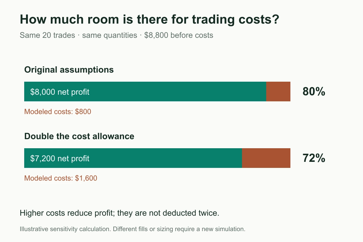
For a strategy with much smaller profits per trade, the same cost change could have a much greater effect on its appeal.

Next, compare with an alternative that serves the same purpose. For a BTC strategy, buying and holding BTC over the same dates is useful context. Compare return alongside drawdown and exposure: a strategy that spends much of the year in cash provides a different experience from holding BTC throughout.

Decide what you want the strategy to contribute. Are you looking for higher growth, less exposure to a falling market, or a source of returns that behaves differently from your other positions? That determines which comparison matters.

2. Translate drawdown into money and time

The path to $18,000 was uneven.

At day 90, the example account reached $13,000. It then fell to $8,800 at day 144 before exceeding the previous peak at day 306.

The decline from $13,000 to $8,800 was $4,200, or 32.3% of peak account value. The peak-to-recovery interval lasted 216 days—roughly seven months.

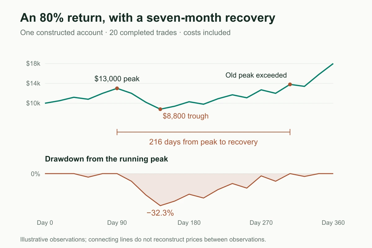
Equity and drawdown use the same constructed observations. Values between observations are joined for illustration; finer observations could reveal deeper losses.

This is where a percentage becomes a personal decision.

If you had allocated $10,000 to this example, could you have stayed with it while $4,200 of peak account value disappeared? Could you have waited seven months to regain that peak? What else would that money have been needed for?

A smaller allocation might make the dollar swings easier to bear. It would not change the strategy’s underlying behavior, and actual costs or minimum order sizes may prevent exact scaling.

Maximum drawdown tells you the deepest decline observed in the test. It is not a ceiling on future losses. Include room for a worse experience when deciding your allocation.

Also inspect open positions. A report that records only closed profits can conceal losses still held in the account. For leveraged strategies, check whether margin and liquidation constraints allow the account to survive the path at all.

3. Read win rate with the size of wins and losses

Our strategy won 12 of its 20 trades: a 60% win rate.

That becomes more useful when we look at the money attached to each outcome.

Profit factor divides total winning P&L by the absolute total losing P&L: $14,800 ÷ $6,800 ≈ 2.18. Here, every dollar lost across losing trades was accompanied by about $2.18 earned across winners.

The average result per trade—often called sample expectancy—is $8,000 ÷ 20 = $400. You can also calculate it from the 60% win rate and the average win and loss.

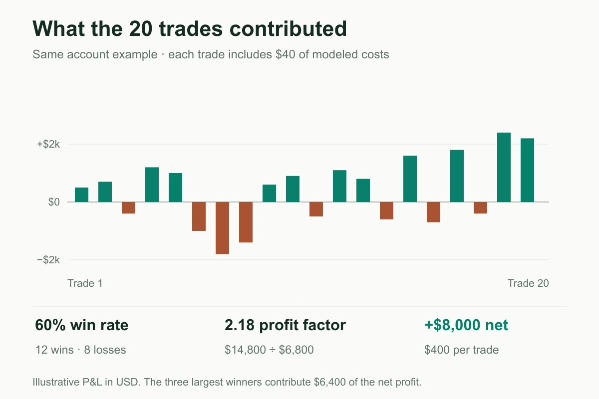
These are the trades used to construct the account curve above. They include $40 of modeled costs per completed trade.

For your own strategy, ask whether its pattern of wins and losses suits you. Frequent small wins with occasional large losses feel different from repeated small losses followed by a few large winners.

Check the definition behind the report, too. A fill count is not a completed-trade count. Profit factor based on closed trades may exclude open losses or costs accounted for elsewhere.

How much depends on the biggest trades?

The three largest winners in our example contribute $6,400 of the $8,000 net profit. Removing their P&L as a diagnostic leaves $1,600.

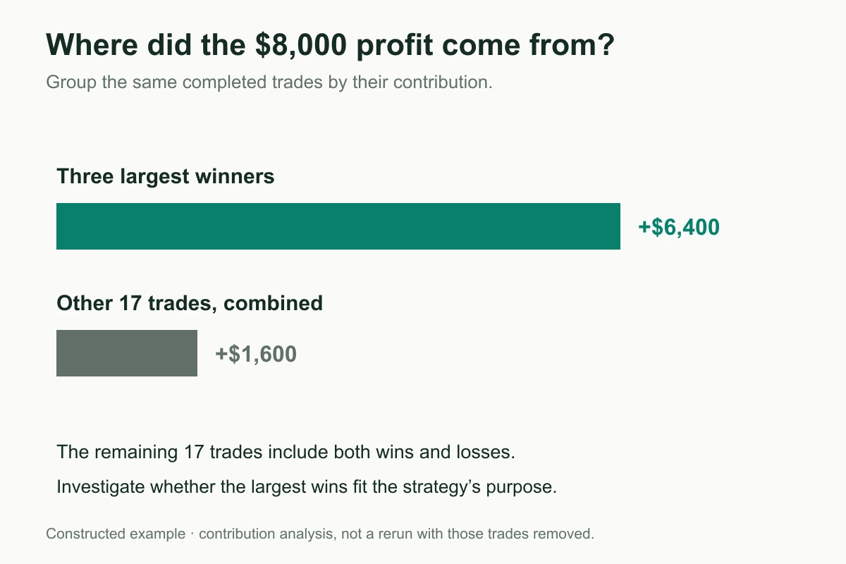
That concentration deserves investigation. A trend strategy may intentionally depend on occasional large moves. You would want to know whether those winners came from opportunities the rules were designed to capture, and whether similar opportunities occurred in other periods.

There are only 20 trades here. The 60% win rate and $400 average describe this sample; they provide limited evidence about what the next 20 trades will look like.

The practical response is to inspect where the profits came from and decide what additional evidence you need.

4. Use Sharpe, Sortino, and Calmar to compare the ride

Return and drawdown are a useful starting point. Risk-adjusted ratios add another view when you compare strategy versions or alternatives.

Sharpe usually measures returns above a risk-free or other reference rate. Some platforms assume that reference is zero. A Sharpe of 1 calculated from one convention is not automatically equivalent to 1 calculated from another.

Sharpe includes both upward and downward variation. Sortino focuses on returns below a chosen target. Calmar connects compounded growth to the deepest observed drawdown.

For the example above, we have shown selected account observations rather than a full daily return series. We therefore do not assign it a daily Sharpe or Sortino from the trade bars. Trades have their own timing and duration; a trade-P&L distribution is not the same as a regularly sampled account-return series.

When you review your own report, compare ratios calculated consistently. A higher Sharpe can make a version worth examining, but also look at whether it reduced exposure, increased turnover, or changed the way returns were distributed.

Avoid treating a particular ratio as automatic approval. A strategy’s role in your portfolio and the evidence behind the estimate matter as much as the headline value.

5. Decide how much confidence to place in the result

Our example earned money after its cost allowance, had a substantial drawdown, and relied heavily on a few winners. That is enough to identify the next questions.

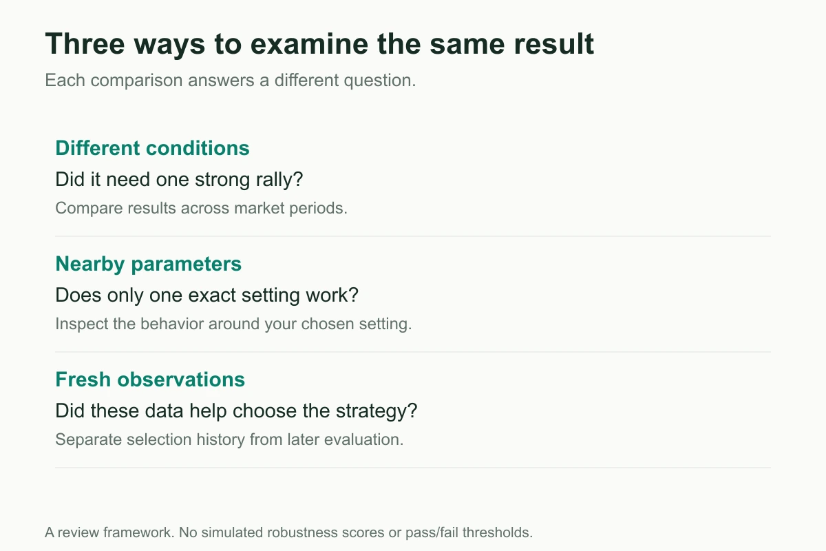
Did it need one particular market?
Split the result by meaningful periods. Find out whether it earned most of its money during a strong rally and how it behaved when prices moved sideways or fell.

Did one exact setting produce the result?
Inspect nearby parameter choices. An isolated optimum deserves more investigation than a range of settings with similar behavior. You are looking for an explanation of the result, including the trade-offs created by the settings.

How many versions were tried?
A strategy selected from hundreds of combinations has had many chances to look good. Keep that search in mind when judging the winning number.

What happened on data that did not help choose the strategy?
A separate evaluation period gives you another observation of the rules. Once you repeatedly adjust the rules after seeing that period, it becomes part of development too.

These questions help distinguish a promising first result from a result you understand well enough to operate. They do not require a statistical research project before you can begin learning from the strategy.

The research behind the search question is discussed in Bailey and colleagues’ Probability of Backtest Overfitting. Kevin Davey’s Don’t Build a Better Backtest gives a practical explanation of how repeated tuning can improve a historical result without improving the strategy.

What would you do with this result?

For someone who needs predictable access to the capital, the example’s seven-month recovery may be too long. Another trader might accept the swings for a small allocation, but want to understand whether the three biggest winners can recur. The same report can reasonably lead to different decisions.

When the result fits your circumstances well enough to explore further, put it into paper trading and focus on what you still want to verify. Once those questions are answered sufficiently, you can decide whether to move to live trading at an allocation you are comfortable with.

As it runs, review the behavior and any parameter adjustments together. Keeping a note of what changed and when helps you understand the results that follow.

A backtest describes historical behavior under its assumptions. Live outcomes can differ. Its value is that you now have concrete evidence—and concrete questions—to guide your next decision.

Review your result with Hetty

Bring those questions to your own strategy.

With HeyTraders, you can describe an idea to Hetty, backtest the rules, and inspect the resulting account curve and trade history. Start with a question that helps you decide what to do next:

Where did this strategy’s profit come from, and what was its hardest period? Show me the drawdown and the trades that contributed most to the result.

You can then explore the costs, allocation, or parameters that matter to your situation. The trading workflow guide explains how that review connects to paper and live trading.

Review my backtest with Hetty